Tile-Based Image Compression

I'm not any kind of data compression expert, but I find the topic quite interesting. There's something fascinating about the idea of data compression and its relationship to machine learning. What I mean to say is that to compress a data stream efficiently, you should ideally capture something fundamental about the structure of the data being encoded. The ideal compression algorithm should somehow be able to "learn" and "understand" the core nature of the data being compressed, so that it can encode it in a very compact way, with as little redundancy as possible. The compression algorithms in use today do this in at a rather superficial level, seeking to shorten the encoding of repeated patterns of bits. LZW, for example, will build a dictionary (a simple grammar) as it encodes a binary data stream, and reuse pieces from this dictionary, when useful, to shorten the encoding. This simple yet clever strategy is remarkably effective, and quite difficult to improve upon.
Image compression is something I find particularly interesting. Images we typically see around, photos in particular, are not at all random. There's structure: edges, shapes, visible patterns and repetitions. Real-world objects, letters, people, curves, textures, all of these things could in theory be mathematically approximated in a way that's much more compact than an array of millions of pixel samples. Our brain is somehow able to recover the underlying structure of the world from images, and transform millions of samples into high-level semantic entities. I've seen people use genetic algorithms to approximate images using colored triangles. This got me thinking: what if you had something more expressive than triangles? Could you use genetic algorithms to evolve boolean functions to encode the pixels of an image as a function of their x/y coordinates?
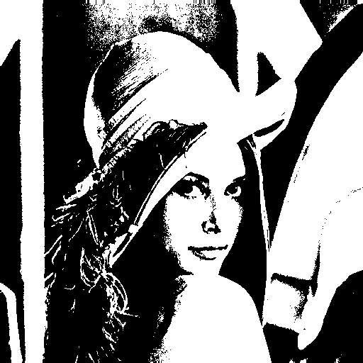
I did a number of experiments trying to come up with boolean functions to approximate one-bit-per-pixel black and white images using mutations and hill climbing, but got surprisingly poor results. There are a number of issues. For one, evaluating complex boolean functions on millions of pixels is very time consuming. Another problem is that there are many complex functions to evaluate, and very very very few of them actually resemble the output we want. It's like looking for a needle in a galaxy. I think that in all probability, an approach using neural networks working with floating-point values would have a better likelihood of panning out. There are training algorithms for neural networks, which would be a better starting point than completely random mutations. Furthermore, floating-point outputs are probably better for learning than boolean outputs, as there are multiple gradations of how wrong a given output is, rather than all or nothing, but this is a topic for another blog post.
After the horrible failure of my boolean image approximation attempt, I sobbed while sipping on one ounce of whisky, but then, I had an idea. Simple approaches that exploit fundamental properties of a problem space tend to do quite well in practice. Maybe something resembling the LZW algorithm would work better. Maybe I could exploit the self-similarity of images (recurring patterns) in a very simple way. I started thinking about an algorithm to encode images using tiles. Split the image into NxN tiles (e.g. 4x4 or 8x8) and encode each tile either as a direct listing of pixel values, or as a reference to another part of the image. The idea is to save space by reusing image information when a similar enough tile already exists. I used the Mean Squared Error (MSE) of tile pixel values to decide when tiles are similar enough to allow reuse. Someone probably has already come up with a similar image compression algorithm before, but my google-fu has not revealed anything obvious.
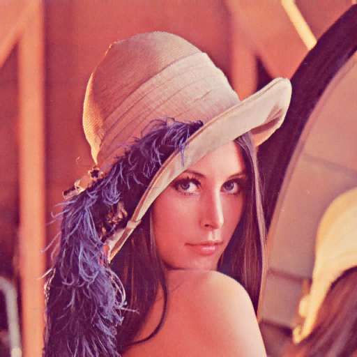
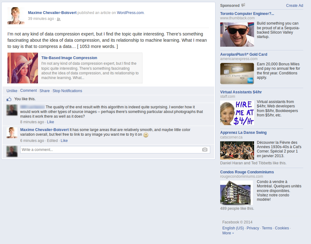
The tile-based algorithm, which my friend Molly has codenamed übersmüsh (USM for short), performs surprisingly well. It's not comparable to JPEG, which is a very sophisticated format layering many levels of clever tricks to get an encoding as compact as possible, but it does much better than I would have expected. Using 4x4 tiles to compress a 512x512 version the classic Lenna image, I was able to generate something visually quite similar to the original by supplying only 610 tiles of source pixel data, out of 16384. This means that only 3.7% of the tiles in the compressed image come from the source image, the rest are all backreferences to x/y regions of the compressed image. I allowed backreferences to rescale the color values of the tiles being referenced for additional flexibility, which makes for a much smaller tile use.
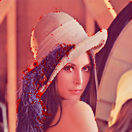
There are some issues, such as the fact that we probably use too few tiles for the background and too many in some detailed regions. This can probably be improved by tweaking or replacing the heuristic deciding when to use source tiles or backreferences. I can think of several other ideas to improve on the algorithm as a whole:
-
Pre-filtering of random noise to make tiles more reusable. The Lenna image has quite a bit of high-frequency noise, as most photographs probably do, due to the nature of image sensors in cameras.
-
Reducing the size of source pixel data using chroma subsampling. This may also have the benefit of making tiles more similar to each other, and thus more reusable.
-
Avoiding supplying whole source tiles and instead supplying only enough source pixels to get an acceptable error threshold. The rest of the pixels would always come from a backreference.
-
Using bigger tiles when possible (e.g. 16x16 or 8x8) and resorting to a recursive subdivision scheme only when necessary. This would reduce the number of tiles we need to encode.
Some important weaknesses right now might be the difficulty of encoding the tile reference table compactly. The code I wrote is also unoptimized and very slow. It's a brute-force search that looks at all possible previous pixel coordinates to find the most-resembling 4x4 tile in what has yet been compressed. This currently takes over an hour on my Code 2 Quad. The algorithm could probably be made much faster with a few simple tweaks to reduce the candidate set size. For example, the tiles could be sorted or hashed based on some metric, and only a few candidate tiles examined, instead of hundreds of thousands. The source code is written in D. It's not the cleanest, but if there's interest I might just clean it up and make it available.
Happy new year to all :)
Edit: Challenge Accepted
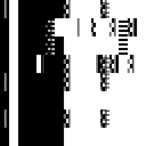
A friend suggested I try übersmüsh on a different kind of image: a screenshot of Facebook containing text and large flat areas. I was curious to see how well it would do, and so I accepted his challenge. I quickly hacked the algorithm to look for matches in restricted size windows (close in position to the current tile). This probably reduces its effectiveness somewhat, but was needed to get a reasonable execution time (minutes instead of multiple hours).

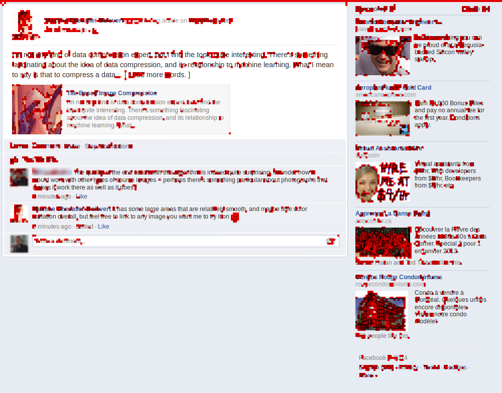
A total of 3354 source tiles was used out of 49000 tiles total, which is about 6.8% of the source image data. Predictably, the algorithm does very well in flat areas. There is some amount of reuse in text, but this could be better if I hadn't reduced the search window size, and instead implemented a better search heuristic. Some of the ad pictures, namely the ones in the bottom-right corner, show very poor reuse, probably because my mean-squared-error heuristic is a poor approximation of what error is visually perceptible.


